The Tail Call Recursion Experiments

I like benchmarking a lot - because it’s very real. We all understand why some algorithm is $O(N^2)$, and the fact that $O(N)$ is better than $O(N\ast lgN)$ and so on. But how do we demonstrate it visually? That’s where benchmarking comes into play.

If computer science were physics, than benchmarking is the experiments to show a theory actually works.

Prerequisite: if you are reading this blog, I am pretty sure you already understand what recursion is. But in case you want to learn more about it - link.

Objective and philosophy

Tail recursion is an optimization used by modern languages to optimize a recursive function - both in terms of runtime and memory. When a recursive function is called, it loads a function call on the implicit call stack. A linear recursive function when called $N$ times, will load $N$ (or $N-1$ depending on how base cases are implemented) function calls on the stack.

In a linear recursive function, when the function is called $N$ times, it will load $N$ (or $N-1$, depending on the implementation of base cases) function calls on the stack, because each function call waits for the previous one to return before completing.

However, things become more complex with N-ary recursion, where a single function call spawns multiple recursive calls (up to $N$ times). This leads to more branching, causing the call stack to grow significantly. Specifically, for an N-ary recursive function, if there are $N$ recursive calls at each level of depth, the number of calls grows exponentially, but the call stack will grow with the depth of the recursion i.e. with $logN$, not with $N^N$.

Hence, some modern languages understand that in some instances actually remembering the function call (by loading it on the stack) is not necessary. It is essential that the recursive function passes any necessary state or calculated values as arguments to the next function call. The function must also return the result of the recursive call directly—without any additional operations or modifications to the return value. If the function needs to perform other computations after the recursive call returns, the compiler cannot apply tail recursion optimization because it must retain the previous call’s state to complete those operations.

Take a look at these two implementations of the Fibonacci function:

Regular (no tail call optimization)

public int fiboRegular(int n) {
    if (n <= 1) {
        return n;
    }
    return fiboRegular(n - 1) + fiboRegular(n - 2);
}

This function computes an entire decision tree to calculate fibonacci of n. Notice how this does not qualify for a tail call optimization, because it break a major rule. Recursive function must return only a single entity - usually the result that it’s computing in the arguments.

Tail call optimized

public int fiboTail(int n) {
    return fiboHelper(n, 0, 1);  // Start with initial values of fib(0) = 0, fib(1) = 1
}
 
private int fiboHelper(int n, int a, int b) {
    if (n == 0) {
        return a;
    }
    if (n == 1) {
        return b;
    }
    return fiboHelper(n - 1, b, a + b);  // Tail-recursive call, no further computation after the call
}

Here, the helper function only returns a single entity, which qualifies for a tail call recursion.

So to sum it up, basically instead of relying on the stack to compute values for us, we rely on the processor’s ability to do math quickly. The compiler/interpreter just reuses the current stack frame and computing argument values. The time taken by a processor to do math is much lower than it’s time taken to access memory.

How are we benchmarking?

Not all languages have the Tail Call Optimization (TCO), hence we have to select a language that does. Many functional programming languages have an incentive to include TCO because there’s no such things as loops - every loop behavior needs to be achieved via recursion.

We use Haskell for the experiment since it’s TCO is very nicely implemented. Haskell is a pure functional language. Haskell has modules such as System.CPUTime that allows use to measure the time taken by a function.

So, we have two implementations of the Fibonacci function - one implemented regularly, and one with Tail Recursion. Since Fibonacci grows exponentially, we have to take smaller values of N or else the regular implementation runs out of stack space very quickly. N = 41 to be exact.

These are the values of N we choose N = (10, 15, 20, 25, 30, 35, 40)

Code

import System.CPUTime
import Text.Printf
 
-- Non-tail recursive Fibonacci
fibNonTail :: Integer -> Integer
fibNonTail 0 = 0
fibNonTail 1 = 1
fibNonTail n = fibNonTail (n-1) + fibNonTail (n-2)
 
-- Tail recursive Fibonacci
fibTail :: Integer -> Integer
fibTail n = go n 0 1
  where
    go 0 a _ = a
    go n a b = go (n-1) b (a+b)
 
-- Timing function that returns the execution time
time :: IO a -> IO Double
time a = do
    start <- getCPUTime
    _ <- a
    end   <- getCPUTime
    let diff = (fromIntegral (end - start)) / (10^9)
    return diff
 
main :: IO ()
main = do
    let n = 10  -- Adjust this value to see more pronounced differences
    nonTailTime <- time $ return $! fibNonTail n
    tailTime <- time $ return $! fibTail n
    
    printf "\nNon-tail recursive Fibonacci(%d) time: %0.6f m sec\n" n nonTailTime
    printf "\nTail recursive Fibonacci(%d) time: %0.6f m sec\n" n tailTime
    
    let speedup = nonTailTime / tailTime
    printf "\nSpeedup factor: %0.2f\n" speedup

PS: the best part is you do not need to setup up a Haskell toolchain on your local machine. Haskell has it’s own playground online that you can use without user authentication. Check it out here: Haskell Playground

Observations

N	Tail Recursion (mS)	Regular Recursion (mS)	Speedup Factor
10	0.001323	0.007444	5.626606198
15	0.001222	0.041429	33.90261866
20	0.009067	0.49205	54.26822543
25	0.01016	5.256463	517.3684055
30	0.022112	29.307847	1325.427234
35	0.011001	360.403672	32760.99191
40	0.010649	3644.321075	342221.9058

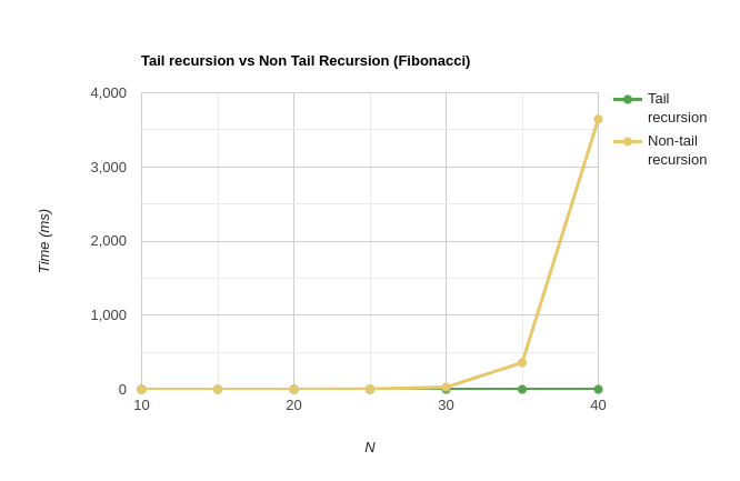
Below is a line graph, of the above data. We can see that the regular recursion is an exponential graph while tail recursion is a linear line. (Note: the tail recursion graph looks constant/logarithmic because of the large range of the data values - but it’s linear)

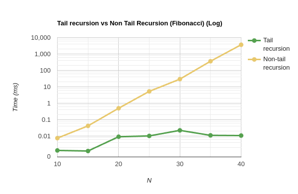
To verify the exponential nature of the graph, let’s convert the scale to logarithmic on the y-axis. This transformation should make an exponential curve appear linear. As we can see, the curve becomes a straight line, confirming the exponential relationship.

Conclusions

Tail recursion is a important optimization implemented by modern languages. It essentially brought down our complexity of the Fibonacci function from $O(2^N)$ to $O(N)$.

Now, was it possible to optimize without tail recursion? Yes. We can use dynamic programming to store already computed results in a memo - hence called memoisation. But that takes extra code and even memory.

— A

GitHub | Twitter